IS GEOCASTING THE NEXT STEP IN CELLULAR V2X COMMUNICATION?
As we enter the era of autonomous driving, sharing information between vehicles has become more important than ever. In the second of our vehicle-to-everything (V2X) blog posts, we discuss the challenges of geocasting, and propose a new geocasting mechanism based on map data that could be the next step for cellular V2X communication.
Sharing information between vehicles on the road is nothing new. Not only does it include safety-related messages linked to icy roads, emergency braking, and other road hazards, but also communication for improving comfort and efficiency by optimizing maneuvers in a collaborative approach and avoiding frequent-stop braking in heavy traffic scenarios.
Some approaches rely on direct communication between vehicles, although this has the general drawback of having limited range because vehicles depend solely on messages sent from other vehicles within its range without any pre-processing.
In a different approach however, vehicles can communicate via cellular networks, such as 5G, reusing existing infrastructure and leveraging on novel developments in edge cloud, protocols on top of IP, and ultra-low latency.
In our previous blog post, Cellular V2X: What can we expect on the road ahead?, we discussed a number of challenges for Cooperative Intelligent Transport Systems (C-ITS) messaging via cellular. One of the challenges is geocasting. We defined geocasting as a routing technique for messages based on the recipient’s geographic area. However, we demonstrated a new geocasting mechanism based on map data that could be the next step for cellular V2X communication. The demo included the distribution of hazard warning messages over cellular communication. The use case was demonstrated in 16 October 2019 in a closing event for the ConVex project using our 5G-Connected Mobility test network on the A9 highway near Nuremberg, Germany.
Identifying the right vehicles
A large segment of automotive services is correlated with the vehicle’s current location and its future path. If we take the Traffic Message Channel (TMC) on the radio as an example, the radio channel broadcasts traffic information related to the region where it is broadcasted, because this is the information that is relevant to the vehicles in this area.
Services offered via IP-based systems use the client IP address to locate it in the network and connect to it. Sometimes the IP address is used to identify the client’s geographical location, since a client IP can tell us in which country the client exists.
How can a service provider or a vehicle identify which vehicles are interested in the information to be distributed? For example, in case of direct communication, the vehicle would broadcast its message, and whoever was in range of that message would be considered relevant.
Going back to the TMC example, the reporter would simply say the following: “For those of you heading south on I-15 on your commute home from work, expect some delays around the 215 interchange. Road crews are making repairs in the left lane, so commuters should be prepared to shift over to the right around 7200 South.” The drivers listening to the broadcast would use their cognitive ability to understand if this information is relevant to them or not. Then they will react accordingly. Unfortunately, such cognitive ability doesn’t exist in vehicles. So, once an incident is identified, it’s crucial to identify how to send a notification to vehicles in the region of the incident. Such knowledge might be difficult for a vehicle to acquire, because it has to track all vehicles in proximity and identify which vehicle has an interest in the information before sending it. That’s why it’s more realistic to delegate this functionality to a node hosted in the cloud.
In the coming sections, we discuss an efficient geocasting algorithm that clusters vehicles according to their locations and distributes messages to vehicles registered to the cluster.
Setting the scene for geocasting
Geocasting is a term used to refer to the process of sending a message to a group of receivers present in a specific geographical cluster. The objective of a good geocasting mechanism is to guarantee efficient distribution of messages to all relevant receivers with the lowest cost possible. So, how do you form efficient clusters, and how do you decide when a vehicle is eligible to join or leave another cluster? It depends on the current location of the vehicle, and its anticipated path.
One easy way to do this is to draw an elliptical area around the vehicle. Once any vehicle enters this ellipse it becomes a member of the cluster. Another way is using a Quadtree data structure to represent a hierarchal decomposition of an area into small regions. This solution was used in the C-roads project and was described in detail in the deliverables. The process of mapping areas into logical clusters is known as geo-referencing. We will also refer to each cluster as the Region of Interest (RoI).

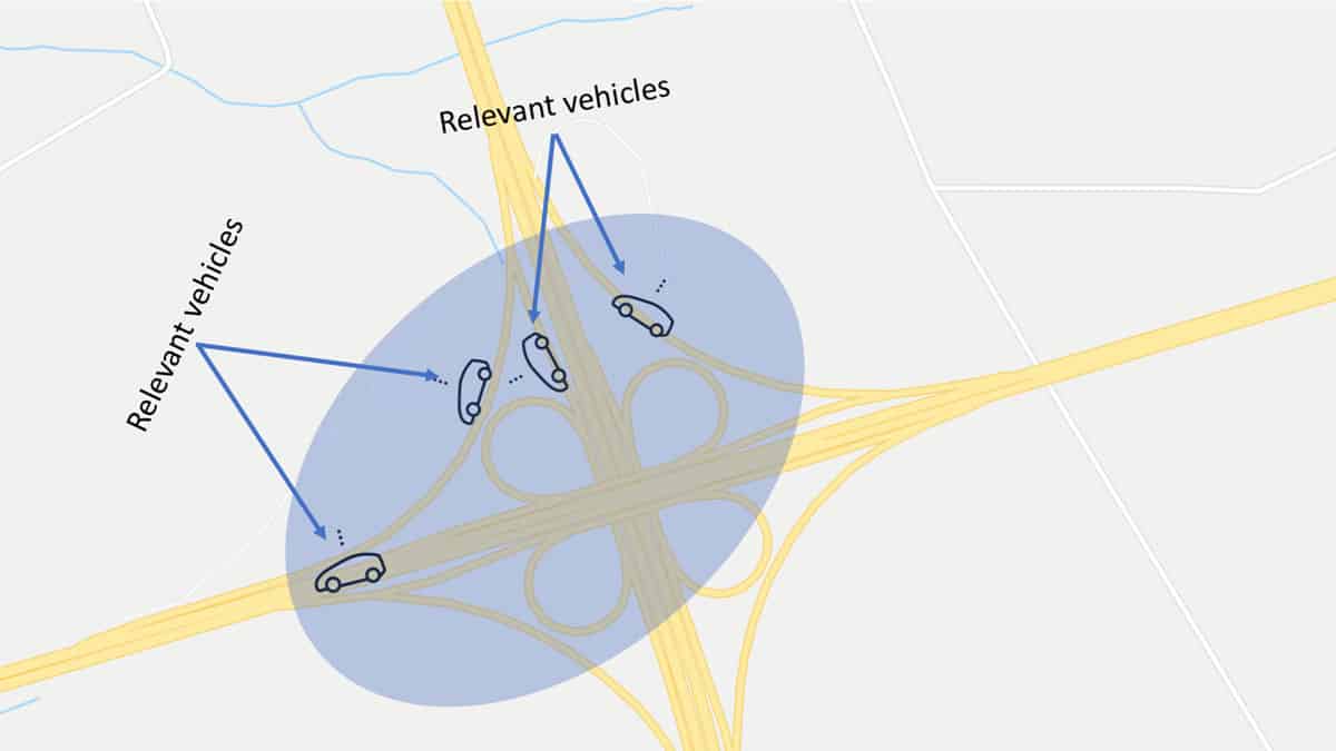
Figure 1: Elliptical Geocasting (Google map data © 2020).
A vehicle or a cloud service can send messages to other vehicles within a given RoI that are not interested in the information. Those vehicles would simply evaluate the message and decide to ignore it. However, this solution might be costly if we use cellular unicast communication because the message was sent to irrelevant recipients.
The street geometry and driving rules are very important factors to determine the RoI. For example, RoI on a highway can be a few kilometers, because of the speed of the vehicles, while on a small street it can be less than 1km. The proposed mechanism uses information derived from map providers such as OpenStreetMap®(OSM) and a set of data structures and algorithms from graph theory to build the RoIs and traverse through them.
Nodes and Ways
If we take a look at a map example from OSM, we will see that it comes in the form of an XML file. It consists of many elements that describe all the details on the map in a given area. The two important elements are Nodes and Ways. Figure 2 represents the nodes in the Map XML. Each node is a virtual point on the map, which has a unique ID and coordinates. This node is used as an anchor point on the map.
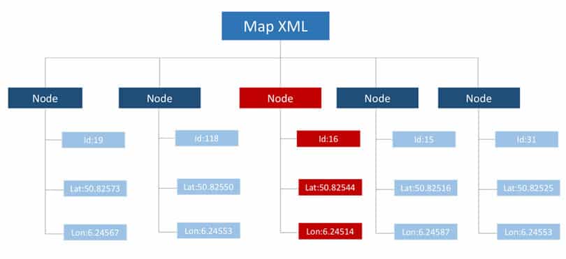

Figure 2: Nodes in the map XML file.
Figure 3 depicts the “Way” representation in the Map XML. It is an element that describes any shape in the Map. This shape could be a building, a garden or a street. Each way consists of multiple elements, where each element has ID reference to a given node. The node references are inserted in the same order where they exist on the street, hence the first node reference in the way element is the first node in this section of the street, and the last node in the element is the last node in this section in the street. The same node can be used to describe multiple ways. If a node exists in two ways that means that this node connects them. As shown in figure 3 and 4, way ID 98555 and way ID 98554 starts and ends at node ID 16 respectively. So, we can say that they are connected via node 16.

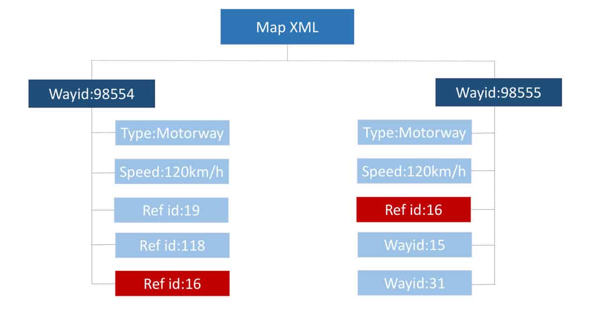
Figure 3: Ways representation in the map
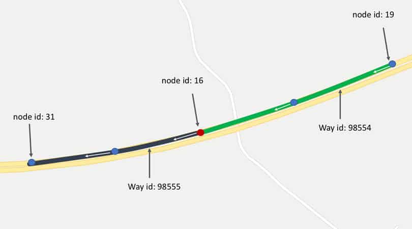
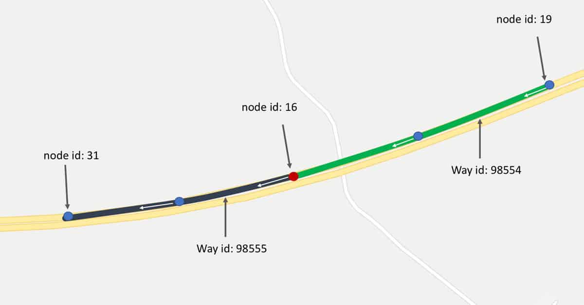
Figure 4: Ways constructed from a group of nodes (Google map data © 2020).
Weighted directed graphs
Using all the nodes, we can build a weighted directed graph. Each node is considered as a vertex, the edge is the line between nodes and the weight is the distance between each node. After forming the graph, we can traverse through it and form a unique RoI out of a group of connected edges.
Each RoI can have a certain shape and length that can be pre-configured. For example, if the edge type is a motorway, we can have each RoI with a length of 10km, while if the edge type is a residential road, we can configure the RoI length to 1km. Beside street speed limit, other factors can also be used to define a suitable length of an RoI such as normal street capacity and network conditions. In principle, the RoI length can range from a few meters to multiple kilometers.
Let’s take a look at figure 5 and observe how our graph looks. We can see that the RoIs are following exactly the same shape as the street. They are also connected to each other in a consecutive way, exactly as the streets are connected in reality. This connectivity is a basic characteristic of graphs which we can use to our advantage to distribute messages in specific areas. For example, if an incident occurs at RoI #3, this would affect all vehicles arriving in this location after 10 km. We can use different graph traversal algorithms to find all RoIs that are 10km away from the incident. If we assume it’s right-hand traffic, it would be RoI #3, RoI #2, RoI #1 and RoI #7. Therefore, all vehicles within those RoIs should get a notification about the incident.
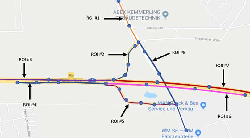

Figure 5: RoI built through a weighted directed graph (Google Map data ©2020)
Now that we partitioned our map into accurate RoIs, how can we find the suitable RoI for each vehicle? We can do this by finding out the closest node to the vehicle. This can be achieved using a space-partitioning data structure such as k-d tree. This allows us to search for the closest nodes to a given point in logarithmic running time, relevant to the number of nodes in the tree. We use it to sort all the nodes used to build the RoI graph based on the coordinates.
Setting the right orientation for nodes
Now that all the nodes are sorted, we can easily query the closest node to our vehicle and figure out which RoI belongs to this node. However, is it always the closest node that is the right node for the vehicle? Not really. What if the closest node to the vehicle is a node in the opposite direction of travel? To solve this problem, we need to identify an orientation for every node. The orientation is the bearing angle between the node and the next node in the direction of travel. That means that a node can have multiple orientation angles if it is on a junction, as shown for node 8 in figure 6, where the bearing angle is the angle between two points and the true north in degrees.
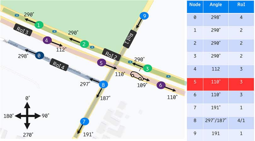
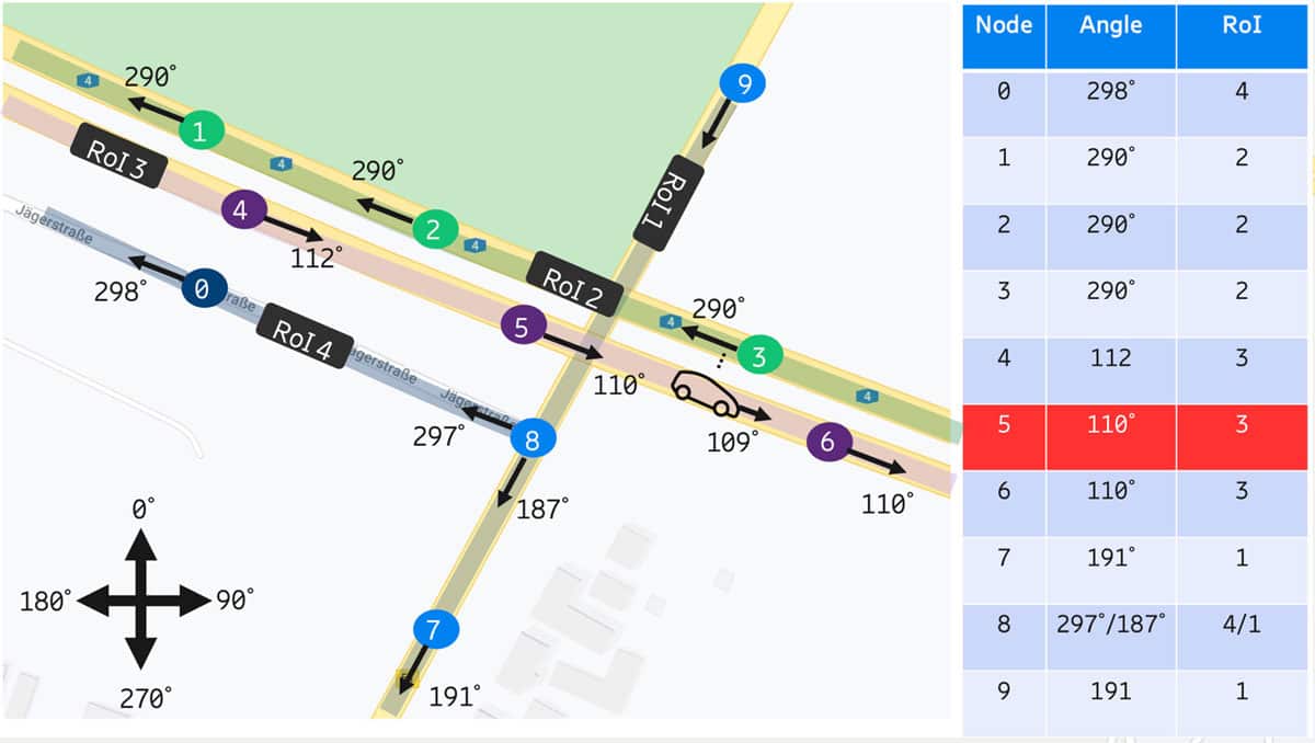
Figure 6: Calculation of the bearing of every node (Google Map data ©2020)
Now that every node has an orientation. We can query the closest 10 nodes to our vehicle. Then we compare the orientation of the closest node to the heading of the vehicle. Here, we need some tolerance because the orientation angle will never be exactly equal to the vehicle heading. Therefore, we need to allow a margin of error of around 10°. If the node is close to the vehicle and has a similar orientation, then the vehicle belongs to the same RoI as the edge corresponding to this node, in case a vertex belongs to two edges, the edge coming to the vertex is chosen.
The geocasting process
Now let’s go over a quick example to see how the geocasting works. Figure 7 shows an abstract call flow for the geocasting process. The geocasting engine is hosted within the application server (AS) process in a pre-configured map area and computes all the RoI graphs and the k-d tree.
The application server exposes an API (Application Programming Interface) for the RoI queries and an API for message distribution. The vehicle sends a query to the application server, including its current coordinates and heading angle. The application server calculates the relevant RoI and identifies its border, both of which are then sent to the vehicle. The application server registers the vehicle in the given RoI. If the vehicle diverts from the RoI, it queries a new RoI. If a vehicle or a service provider detects an incident, it sends the incident message to the application server including the hazard coordinates, the direction of travel and the range of the message distribution (i.e., how far the message should be sent from its source). The application server calculates the current RoI of the message, just like it would do for a vehicle. Afterwards, it traverses through the graph and finds all connected RoIs within the range. Finally, the application server forwards the message to all vehicles that are registered to the targeted RoIs.
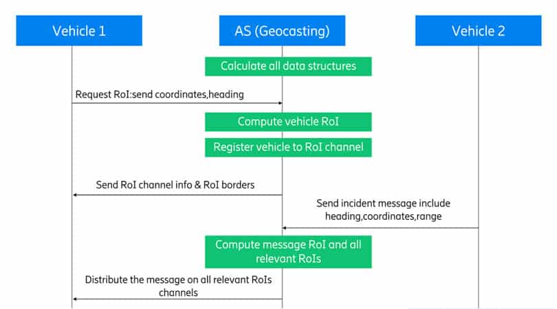

Figure 7: Abstract call flow for the geocasting APIs
It can be noted that the call flow described in figure 7 represents an abstract call flow using the proposed API. With few modifications, it can be applied for protocols with a publish/subscribe pattern such as Message Queuing Telemetry Transport (MQTT) or pull pattern such as HTTP or even a combination of different patterns.